Table of Contents
Looped transformers promise more computation without proportionally more parameters. While reading the Huginn paper, I wondered what parameter sharing means for GPU memory. Does reusing the same parameters avoid additional HBM traffic by keeping them in on-chip caches. The short answer is that sharing weights reduces the amount of parameter data a model needs to store. But it does not automatically reduce how much data the GPU reads from HBM. In this post, I explore when shared weights can be reused from cache and when they must be read from HBM again.
The idea of recurrent depth predates Huginn — Universal Transformers explored shared-weight recurrence in 2018. In this post, I use teaching implementation of Huginn’s public inference code with random weights as a concrete case study.
Chapter 1 - What Repeats?
So how does looped Transformer differ from standard Transformer? A Standard Transformer usually uses separate parameters for each layer. A Looped Transformer repeatedly applies same group of layers, reusing their parameters. In Huginn, the repeated part is called Core This way of reusing parameters adds computation without adding another set of Core parameters. However, sharing parametres still doesnt mean less computation at every iteration.
The diagram below shows the main difference between standard and looped Transformers:
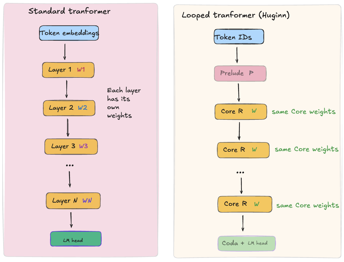
Prelude, Core, and Coda
From diagram above you could notice that Huginn organizes its forward computation into 3 stages: Prelude, Core and Coda (shown in the diagram below).
Prelude - prepares the input representation e, which stays fixed throughout the Core iterations of the current forward pass.
Core - this stage starts from a randomly initialized current state s₀. Next, at each iteration shared adapter combines the current state s with fixed input e. Then four Transformer layers produce the updated state s_{i+1}. Each layer uses causal attention with RoPE, a gated SiLU MLP, residual connections, and sandwich RMSNorm. Each Core layer has its own parameters and reuses them across iterations. A Core iteration updates the hidden state; it doesn’t generate a new token by itself.
Coda - after the final Core iteration, processes the final recurrent state. The LM head then produces vocabulary logits to select the next token.
Both e and s_i contain one hidden vector per processed token position.
Here is the diagram of Huginn’s recurrent-depth architecture.
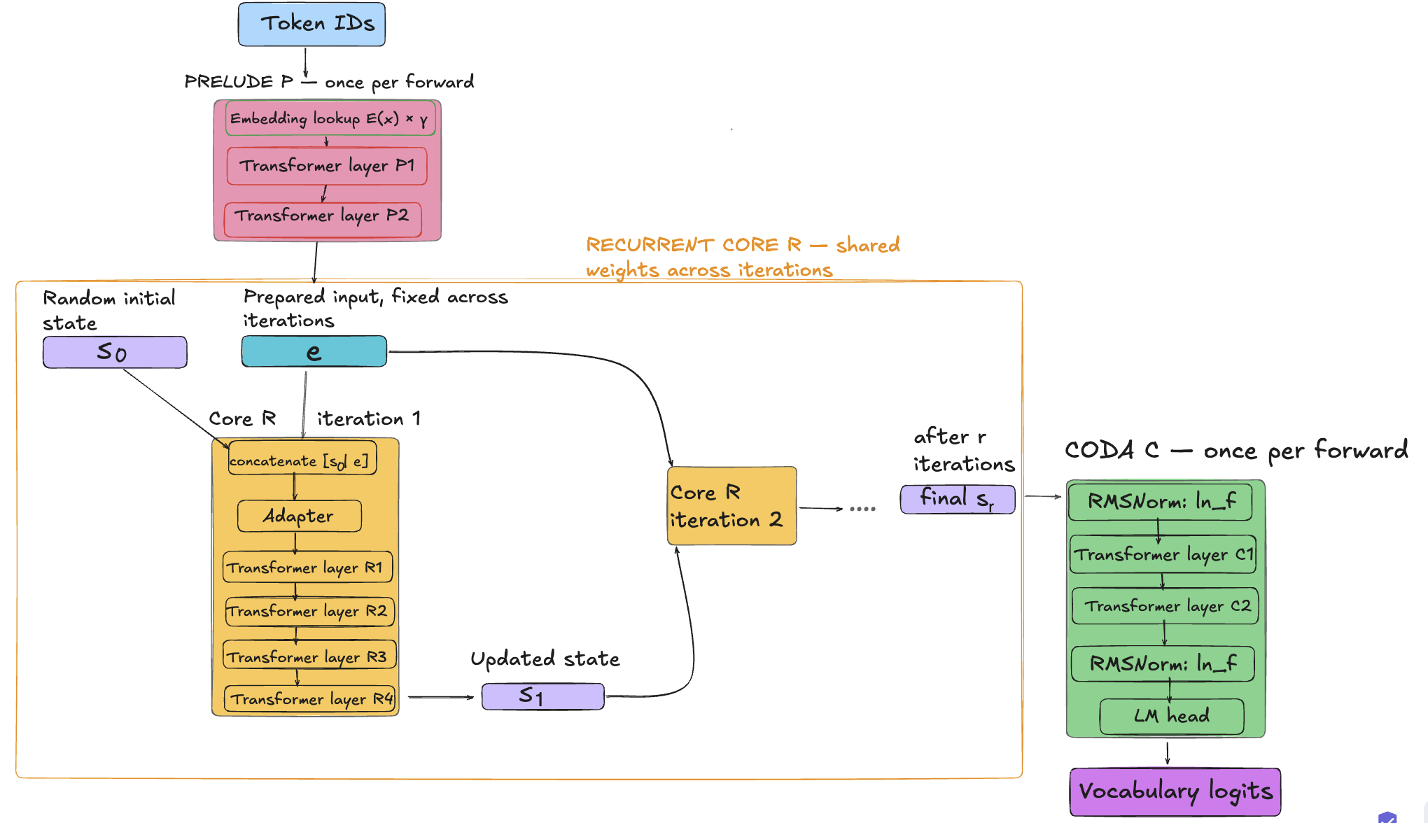
As you can see inside one Сore R iteration we have 4 Transformer layer R1, R2, R3, R4 - each has its own parameter set. However R1 uses the same R1 weights at every Сore iteration, and this works not only for R1 but for other layers and adapter too. These parameters stay fixed while the hidden state is updated.
In simplified pseudocode, the forward pass can be represented like this:
e = prelude(tokens)s = random_state_like(e)
for step in range(num_iterations):    s = core(s, e)  # Shared weights across iterations
logits = lm_head(coda(s))
Shared weights don’t mean shared KV across iterations. With a full KV cache each Core layer keeps a separat KV cache for every iteration. Increasing the iteration count therefore increases Core KV-cache storage, even though Core parameter storage stays fixed.
I use BF16 and a fixed number of iterations, full recurrent KV cache, without early exit or cache sharing. The Core benchmarks use a teaching implementation with random weights, not the complete trained Huginn model.
Well, now we know what repeats, what parameters are shared and what is not. Weight sharing can reduce parameter storage, but my question is does it also reduce the number of bytes moved from HBM or the time required to execute the model?
Chapter 2 - What Should One Core Iteration Cost ?
To understand what sharing weights costs on GPU, we need to clarify 3 quantities:
- Storage: how much memory the tensors occupy.
- Computation: how many operations we perform.
- Traffic: how many bytes move between GPU memory and the processors.
A weight matrix can occupy memory once but be read many times. Sharing parameters therefore does not automatically reduce memory traffic. Below, I estimate these quantities for one Core iteration and use them to reason about execution time. Later chapters compare these expectations with measurements.
I assume you are familiar with prefill and decode. If not, I explain them in Appendix A.
One Core Iteration cost
I apply these quantities to every operation in the recurrent Core. The tables below show costs of the adapter, four attention modules, four MLPs, and their normalization parameters.
I use Huginn’s configuration: hidden size 5,280, MLP intermediate size 17,920, and 55 attention heads of dimension 96. Inputs and weights are BF16, and attention is causal. Batch size is one. Prefill processes 1,024 positions; decode processes one new position with 1,024 cached positions.
Parameter Storage:
| Core component | BF16 parameter storage, MB |
|---|---|
| Adapter | 111.514 |
Attention projections: QKV + Wo | 892.109 |
| MLP | 2,270.822 |
| RMSNorm scales and Q/K biases | 0.253 |
| Complete Core | 3,274.698 |
Work counts include matrix multiplications only. Attention counts include only causally allowed query–key pairs; softmax and other operations are excluded.
Useful Matrix-Multiplication Work:
| Core component | Prefill, GFLOPs | Decode, GFLOPs |
|---|---|---|
| Adapter | 114.190 | 0.1115 |
Attention projections: QKV + Wo | 913.519 | 0.8921 |
| QK + PV | 44.335 | 0.0866 |
| MLP | 2,325.322 | 2.2708 |
| Complete Core | 3,397.367 | 3.3610 |
At this context length of 1,024 positions, the MLP takes most of the recurrent Core’s parameter storage and counted FLOPs. These counts alone do not tell us which operation takes the most time.
Roofline Estimate
The tables above give the weight bytes and the FLOPs of one Core iteration. To turn them into a rough time estimate, I divide the FLOPs by the GPU’s peak compute throughput and the bytes by its peak HBM bandwidth. This is a simple roofline model:
Compute time = FLOPs / peak compute throughputMemory time  = assumed HBM traffic / peak HBM bandwidth
Ideal time ≈ max(compute time, memory time)
I count only the weights as HBM traffic. Based on NVIDIA’s published specifications, I use peak limits of 2,250 TFLOP/s for dense BF16 and 8 TB/s for HBM bandwidth for one B200.
| Mode | FLOPs per iteration | Weight bytes | Compute time | Memory time | Ideal time | Limited by |
|---|---|---|---|---|---|---|
| Prefill, 1,024 positions | 3,397 GFLOPs | 3.275 GB | 1.51 ms | 0.41 ms | 1.51 ms | Compute |
| Decode, 1 position | 3.36 GFLOPs | 3.275 GB | 0.0015 ms | 0.41 ms | 0.41 ms | HBM bandwidth |
If every iteration reads the Core weights from HBM again, 32 iterations read about 104.8 GB of weights, while the parameters still occupy only 3.275 GB. At 8 TB/s, these reads alone take at least 13.1 ms for every generated token.
This model assumes that computation and memory transfers overlap perfectly, thats why the ideal time (above) is max between compute time and memory time. Actual execution also depends on kernel efficiency and launch overhead and KV-cache access and intermediate tensors add further traffic. These are back-of-the-envelope estimates. Appendix A checks this way of counting bytes on one operation, the adapter.
However, the memory estimate depends on how many bytes actually reach HBM. That requires measurement. In the next chapter, i test - do shared weight addresses allows data to stay in on chip cache until the next iteration.
Chapter 3 — Do Shared Weights Reduce HBM Traffic?
I compare two versions of the same repeated matrix multiplication. One uses a single weight matrix throughout, while the other uses separate copies containing exactly the same values.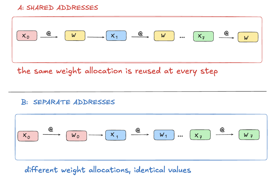
Each version contains eight sequential matrix multiplications. The output of one step becomes the input to the next. The state has shape [1, d], and each weight matrix has shape [d, d].
In A, all steps access the same physical weight allocation. In B, every step accesses a different allocation, but the numbers are identical. Both versions produce exactly the same BF16 outputs.
All weights are already on the B200 before timing. Both versions use BF16 and CUDA Graph replay after warmup. The cache is not cleared, so data can be reused within and between chains. To keep the test simple and focused on weight reads, each step is only a matrix multiplication, with no activations, normalization, or attention. It is a chain of linear operations, not a complete Transformer block.
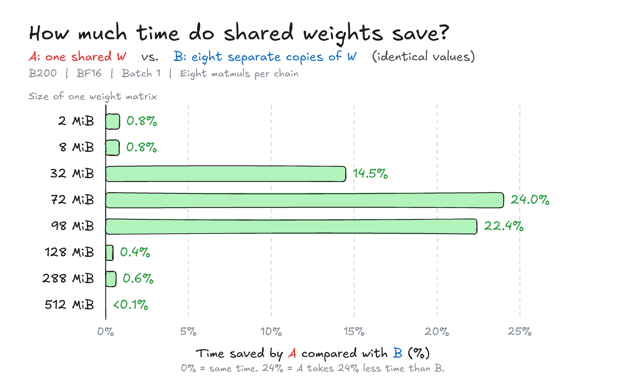
To understand these timing differences, I measured how much data each version reads from HBM.
HBM reads are measured separately with Nsight Compute’s application-range replay and averaged over 100 chains of eight multiplications. The profiler did not clear the cache. The table reports all HBM reads per chain, not just weight reads.
The GPU reports 126.5 MiB of L2 cache. The table shows how much data is read from HBM during eight multiplications:
| One matrix size | A: one shared allocation | B: eight separate allocations |
|---|---|---|
| 8 MiB | ≈0× matrix reads | 0.1× |
| 72 MiB | ≈0× | 8× |
| 288 MiB | ≈8× | ≈8× |
Here, 8× means reading as many bytes as eight full weight matrices. The measurements include all HBM reads, not just weights. Lower values mean less HBM traffic.
At 8 MiB (small working set), both versions benefit from caching. Even eight copies occupy only 64 MiB. After warmup, both generate little HBM traffic, and their execution times are almost identical.
At 72 MiB (medium working set), sharing makes a difference. One matrix fits within the reported L2 capacity, while eight copies occupy 576 MiB. Version A generates almost no HBM reads after warmup and has 24% lower latency. however B version reads approximately all eight matrices. Cache access and computation still take time.
At 288 MiB, the advantage largely disappears. Even one matrix exceeds L2 capacity. Both versions read approximately 8 × 288 = 2304 MiB per chain. Using the same addresses no longer avoids repeated HBM reads in this workload.
The L2 counters show the same pattern. At 72 MiB, the L2 read hit rate was about 100% with shared weights and 4% with separate copies. At 288 MiB, it was about 2% in both cases. These rates include all measured L2 reads, not just weights.
The controlled experiment therefore shows that reusing the same allocation can reduce HBM traffic when reused data remain in L2 until their next acces.
From One Matrix to a Recurrent Core
A real Core performs many operations between two uses of the same weight matrix. Other weights, activations, and KV data also occupy the memory hierarchy. To test this setting, I use a teaching implementation with Huginn’s dimensions and random weights, not the complete trained Huginn model.
Instead of comparing shared weights against separate copies, I compare one Core iteration with eight dependent iterations. The prepared input e stays fixed, while each iteration updates s. Prelude, Coda, and the LM head are excluded. All iterations use the same adapter and four Transformer layers, with separate KV-cache entries for each layer and iteration.
| Mode | One iteration, ms | Expected: 8 × one, ms | Measured eight iterations, ms | Difference |
|---|---|---|---|---|
| Prefill | 4.631 | 37.046 | 36.893 | −0.41% |
| Decode | 1.323 | 10.588 | 10.639 | +0.48% |
Expected times are calculated before rounding.
Under these warmed-up conditions, the average time per Core iteration was almost the same for one- and eight-iteration chains. Parameter storage remained unchanged.
I also measured HBM reads for this Core chain:
| Mode | HBM reads per iteration | Core weights |
|---|---|---|
| Prefill | 4.22 GB | 3.275 GB |
| Decode | 3.39 GB | 3.275 GB |
In decode each iteration reads about as much as all Core weights and eight iterations read eight times as much as one. The weights are stored once, but decode reads about their full size from HBM at every iteration. These counts include all data, not just weights. The benchmark code and full results are available on GitHub.
Each benchmark chain restarts from the same initial state and history. Decode includes history copying performed by the teaching implementation’s torch.cat cache update.
These experiments show that:
- Parameter sharing reduces parameter storage.
- Cache reuse can reduce HBM traffic only while relevent data remains available in L2.
- The Core experiment shows that the average time per Core iteration stayed almost unchanged.
The next question is where reuse can actually happen inside the GPU and why it often ends before the next recurrent iteration.
Chapter 4 — Where Does Reuse Actually Happen?
The previous chapter showed that shared weights can reduce HBM traffic, but not at every tested size. To understand why we need to clarify two things: keeping weights allocated on the GPU and keeping their data close to the processors.
In my expirements weights are already in GPU memory, so we dont move data from CPU to GPU. The question is not whether to copy them from the CPU, but where their next read will be served from.
GPU has different types of memory with different roles:
| Memory | Main role | Data lifetime |
|---|---|---|
| HBM | Stores weights, states, KV cache, and large intermediates | Across kernel launches, until the buffer is freed |
| L2 | Caches recently accessed global-memory data | Cached data may survive across kernels until evicted |
| SMEM | Holds explicitly managed tiles inside a kernel | Until the owning thread block ends |
| Registers | Hold thread-local fragments and temporary values | During the thread’s execution |
| TMEM | Holds Blackwell Tensor Core data, mainly accumulators | Explicitly allocated and freed within a kernel |
Weight sharing allows every Core iteration to use the same stored parameters. It doesn’t guarantee that their data remain in an on-chip cache between iterations. Reuse from L2 depends on cache residency, while SMEM, registers, and TMEM can improve reuse inside a kernel. They do not automatically preserve data across separate kernel launches or complete Core iterations.
A matmul kernel processes weights in tiles, so the whole matrix does not need to fit on chip.
Reusing a weight tile within one matmul is different from keeping it available until the next Core iteration. To illustrate this, let’s look at the diagram of the QKV projection in the first Core layer:
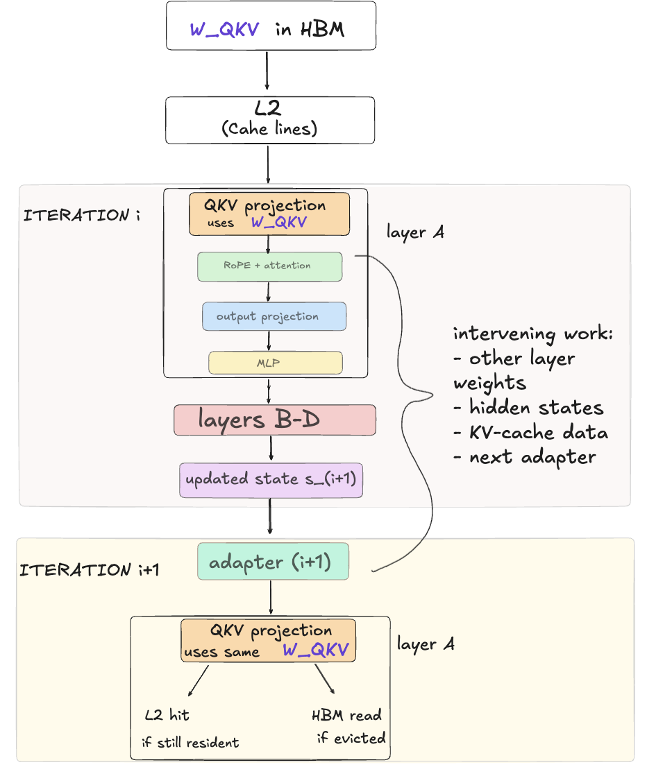
As shown in diagram above you can see that between two uses of the same QKV matrix, the GPU accesses other weights, hidden states, attention inputs and outputs. L2 has limited space, so these accesses can replace data previously loaded into the on-chip cache. If a needed weight tile is no longer cached, the GPU must read it from HBM again.
This explains why efficient tiling within a matrix multiplication does not guarantee that weights remain cached across Core iterations. What matters is not just the size of one matrix, but also the data accessed before that data is needed again.
There are three reasons why we cannot simply keep all the Core’s data on chip between iterations:
- Capacity - our Core contains approximately 3.275 GB of BF16 parameters. On-chip storage is much smaller (tested B200 reports 126.5 MiB of L2). Keeping selected tiles nearby is practical but keeping the entire parameter set there is not.
- Lifetime - in PyTorch implementation, a Core iteration launches many CUDA kernels. The next iteration launches those operations again. The previous kernels’ shared-memory tiles, register values, and TMEM contents are not automatically available to the next recurrence
- Dependencies - next iteration consumes the updated state produced by the previous one. We cannot simply load one weight tile and independently perform all iterations with it because of required inputs depend on other operations that have not yet finished.
Pipelining can overlap the loading of a new tile with computation on the current tile, but it does not remove the transferred bytes. Similarly, shared-memory swizzles and CTA cooperation can improve the execution of individual kernels without making the complete Core persistent across recurrent iterations.
The controlled experiment showed that reusing one physical weight allocation reduced HBM traffic only when it enabled L2 cache reuse, but provided almost no traffic advantage for the largest profiled matrix. Weight sharing therefore creates an opportunity to move fewer bytes, but the memory hierarchy and execution schedule determine whether that opportunity becomes a speedup.
A looped Transformer reuses parameter addresses by construction. Efficient tiling can reuse loaded data within a kernel, but it does not guarantee that those data will remain on chip until the next Core iteration.
Chapter 5 - Conclusion
Sharing weights reduces the amount of parameter data a model needs to store. But it does not automatically reduce HBM traffic or execution time.
Our controlled matrix experiment showed both outcomes. After warmup, the shared 72 MiB matrix generated almost no HBM reads, and its eight-step chain took 24% less time than the version using separate copies. At 288 MiB, both versions read almost the same amount of data from HBM.
In the teaching Core, eight iterations took almost eight times as long as one. The weights were shared, but each iteration still performed its computations. HBM reads followed the same pattern - eight iterations read almost eight times as much data as one. These measurements include weights, KV-cache data, and intermediate tensors, not just weights.
These experiments used random weights on one B200, not the complete trained Huginn model. They do not establish whether additional iterations improve model quality.
The main takeaway is that sharing parameters and reusing cached data are different things. Reusing the Core avoids storing another set of weights, but each additional iteration still performs computation. In our experiments sharing weights reduced HBM traffic when the GPU could reuse those weights from cache.
Appendix A: Prefill and Decode
Prefill processes all positions in the prompt together and builds their KV cache. Decode processes one new position per sequence, using the cached keys and values from earlier positions. Both use the same weights, but process different amounts of input data. This difference mainly affects how those weights are reused during computation.
In this post, batch size is one. Prefill processes 1,024 positions; decode processes one new position with 1,024 cached positions.
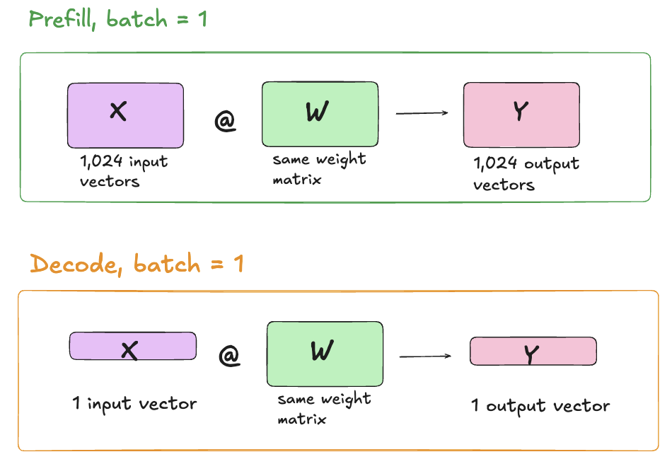
The same linear layer during prefill and decode.
The adapter as a worked example
The adapter is the simplest operation in the Core, so it shows the difference between the two modes clearly.
The adapter was introduced in Chapter 1 as the first step in Core iteration. Adapter combines the current state s with a fixed Prelude output e, increasing the hidden width from h to 2h, and a learned linear projection returns the result back to h. The same adapter weights are used at every iteration.
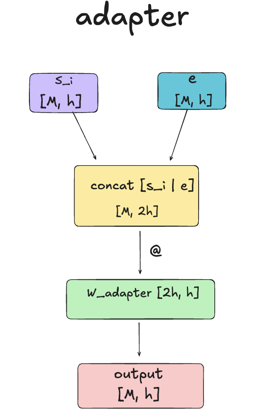
The adapter computes:
[M, 10560] @ [10560, 5280] → [M, 5280]Here, M is the number of positions processed together: M = 1024 for prefill and M = 1 for decode. The weights are shown in mathematical multiplication order.
| Prefill | Decode | |
|---|---|---|
| Input after concatenation | [1024, 10560] | [1, 10560] |
| Weight matrix | [10560, 5280] | [10560, 5280] |
| Output | [1024, 5280] | [1, 5280] |
| BF16 parameter storage | 111.514 MB | 111.514 MB |
| Useful matmul work | 114.190 GFLOPs | 0.111514 GFLOPs |
| Estimated HBM reads | 154.767 MB | 111.556 MB |
| Estimated HBM writes | 32.440 MB | 0.032 MB |
| Measured HBM reads, cold L2 | 160.742 MB | 111.773 MB |
The estimate counts one HBM access for each required tensor read or write, including a separate concatenation operation. To check it, I measured one adapter call on the B200 with Nsight Compute. Before each measured call, I clear the L2 because in the recurrent Core four other layers run between two adapter calls. In decode measured reads match the estimate within 0.2%: almost all of them are the weight matrix. In prefill, the GPU reads about 4% more than estimated; the counters dont show which data was read twice. I dont compare writes, because some written data is still in L2 when the measurement ends. Full results.
The key difference is that prefill performs 1,024 times more matrix-multiplication work than batch-one decode, using the same weight matrix. Parameter storage is fixed, but the amount of computation and ways for weight reuse change.
Roofline for the Adapter
As an example, i take the adapter matmul alone, excluding concatenation. Assume that it reads the weights and input from HBM once and writes the output once. Based on NVIDIA’s published specifications, I use peak limits of 2,250 TFLOP/s for dense BF16 and 8 TB/s for HBM bandwidth for one B200. These are theoretical peak limits.
Roofline estimate for the adapter matmul:
| Mode | Estimated arithmetic intensity, FLOP/byte | Ideal roofline ceiling, TFLOP/s | Predicted regime |
|---|---|---|---|
| Prefill, 1024 positions | ≈793 | 2,250 | Compute-bound |
| Decode, 1 position | ≈1 | ≈8 | HBM-bandwidth-bound |
Under these assumptions, prefill is limited by computation, while batch-one decode is limited by HBM bandwidth.
I also timed the adapter matmul on the B200. Decode took 24.4 µs instead of the ideal 13.9 µs, and prefill took 81.4 µs instead of the ideal 50.8 µs. In both modes the real kernel reaches only about 60% of the roofline limit.